Computer modeling of machine parts
22. Apríl, 2011, Autor článku: Vondřich Jiří, Strojárstvo
Ročník 4, číslo 4  Pridať príspevok
![]() The article describes a computational modeling machine and its parts. For example, the appropriate procedure, numerical solutions and the comparison with the calculation carried out analytically are described. The general procedure is to create an appropriate model, determining the number of degrees of freedom, the mathematical description (at the discretion of the weight and geometric quantities, types of movements, types of strain, the type of drive and load, respectively other parameters).
The article describes a computational modeling machine and its parts. For example, the appropriate procedure, numerical solutions and the comparison with the calculation carried out analytically are described. The general procedure is to create an appropriate model, determining the number of degrees of freedom, the mathematical description (at the discretion of the weight and geometric quantities, types of movements, types of strain, the type of drive and load, respectively other parameters).
The resulting equations are then solved numerically by the program Matlab. As an example, it is stated in the article the numerical solution of plane stress distribution of rotating wheel. The result is the calculation of a radial and tangential stress σr, σt for each disc form. The simplest shape is the wheel disc of constant thickness (example 1).
Another form of N wheel divides the cylindrical rings and is determined by calculating the voltage on the outer ring, which is the default stress of the next ring (example 2). The replacement profile side wall ring hyperboloid refines the previous calculation and the normal stress and tangential stress σr, σt is along the increasing radius of the smallest disk (example 3).
The constantly increasing speed of the rotating parts of the machinery, increasing normal stress and tangential stress σr, σt. This article aims to show the possibility of a suitable design model disc form and numerical solution of the normal stress and tangential stress are at a minimum.
1. Introduction
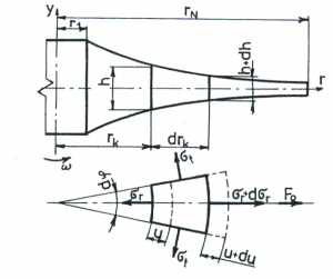
Of the known boundary values of the hyperbolic k-th ring (Fig. 1) is calculated for the change of its thickness h are
| (1) |
where exponent of the hyperbola b is
| (2) |
where value for the exponents b are for the ring: constant thickness b=0, widening b>0 and narrowing b<0.

Figure 1: The out of joint element profile wheels
2. Calculation of stress σ and deformation u
Under the terms of the balance of forces in r direction (Fig. 1) we obtain
| (3) |
Editing (3) we obtain
| (4) |
where ρ is density and ω is angular velocity. The strains are defined
| (5) |
where u is deformation. μ is Poisson’s ratio. and generalized Hooke’s law [1] is
| (6) |
Where μ is Poisson’s ratio. The equations (4), (5) can be calculated
| (7) |
Substituting (7) into equation (4) we obtain for k-th ring true
| (8) |
where E is Young’s modulus. Substituting (7) into equation (4) we obtain
| (10) |
solution of the equation (10) is deformation
| (11) |
Substituting (11) into (7) we obtain
| (12) |
We calculated the constants C1, C2 from the boundary conditions
| (13) |
where p1, pN are known pressures on the wheel radius r1, rN (Fig. 1)
3. Results
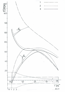
With Matlab [1], [2], [3] it is possible to calculate curves σr, σt for examples 1, 2, 3 (Fig.2). Parameters are the wheels:
,
,
,
,
,
,
,

Figure 2: The stress σr, σt for examples 1, 2, 3
The curves in Fig. 2 show that the tension is the smallest at the wheels with the hyperbolic profile.
References
- B. Doňar, K. Zaplatílek. MATLAB pro začátečníky, 1 díl, BEN, Praha, 2003
- B. Doňar, K. Zaplatílek. MATLAB- tvorba uživatelských aplikací, 2. díl, BEN, Praha, 2004
- B. Doňar, K. Zaplatílek. MATLAB- začínáme se signály, 3.díl, BEN, Praha, 2006
Czech Technical University in Prague, Faculty of Electrical Engineering, Department of Electric Drives and Traction, Group Mechatronic

