The focus of this paper is the implementation of a constrained Model Predictive Control algorithm using a Multi-Parametric Toolbox (MPT), which is a free MATLAB toolbox for design, analysis and implementation of optimal controllers for constrained linear, nonlinear and hybrid systems. In this paper, we show how to move all the computations necessary for the implementation of MPC offline by using multi-parametric approach, while preserving all its other characteristics. In the end we demonstrate these methods with designing an optimal controller for some examples.

1. Introduction

Linear systems with input, output, or state constraints are probably the most important class of systems in practice and the most studied as well. Although, a variety of control design methods have been developed for linear systems, the most popular control approach for linear systems with constraints is model predictive control or simply MPC which has become the standard for constrained multivariable control problems in the process industries. Nowadays, MPC approach can be found in a wide variety of applications and this is something that would have been impossible without the development of new, more effective optimizations algorithms.

The idea behind MPC is to start with a model of the open-loop process that explains the dynamical relations among system’s variables (command inputs, internal states and measured outputs). Then, constraint specifications on system variables are added, such as input limitations (typically due to actuator saturation) and desired ranges where states and outputs should remain. Desired performance specifications complete the control problem setup and are expressed through different weights on tracking errors and actuator efforts (as in classical linear quadratic regulation). The rest of the MPC design is automatic.

First, an optimal control problem based on the given model, constraints, and weights, is constructed and translated into an equivalent optimization problem, which depends on the initial state and reference signals. Then, at each sampling time, the measurements of the current output (state) of the system are retrieved and an open-loop optimal control problem is solved over a finite time horizon to obtain the sequence of future control values. The first value of the sequence is then obtained and the procedure is repeated starting from the new state and over a shifted horizon, leading to a moving horizon policy.

For this reason the approach is also called the receding horizon philosophy. The standard on-line solution at each sampling time is not suitable for fast systems, so there has been found a way how to solve the optimization problem explicitly off-line (Bemporad et al., 1999; Borrelli et al., 2001). The explicit solutions to constrained MPC problem increase the potential applications areas for using MPC approach. The Multi Parametric Toolbox (MPT) (Kvasnica et al., 2004) provides the solvers for computing the explicit optimal feedback control laws for constrained linear and piecewise affine systems.

The paper is organized as follows: firstly, the basics of MPC are reviewed to derive the quadratic program which needs to be solved to determine the optimal control action. Next, the multiparametric quadratic programming problem is studied and it is shown that the optimal solution is a piecewise affine function of the state. We analyze its properties and present an efficient algorithm to solve it. The paper concludes with some illustrative examples.

2. Unconstrained optimal control

Consider the problem of regulating the discrete-time system (1) to the origin.

(1)

where x(k)єℝⁿ is the state vector at time k, u(k)єℝ^m is the vector of manipulated variables to be determined by the controller and y(k)єℝ^p is the vector of output variables. The desired objective is to optimize the performance by minimizing the infinite horizon quadratic cost

(2a)

(2b)

(2c)

(2d)

where x_kєℝⁿ denotes the predicted state vector at time t+k obtained by applying to (1) the first k samples of the input sequence u₀,…,u_∞, starting from x₀=x(t); u_kєℝ^m and y_kєℝ^p are the input and output vector, and the pair (A, B) is stabilizable. The tuning parameters are the symmetric matrices Q≽0 (positive semidefinite) and R≻0 (positive definite) corresponding to weights on state and input. It is also assumed that the pair (√Q, A) is detectable. When no constraints are considered, the infinite horizon objective (2) could be minimized by the time-invariant state feedback

(3)

where the matrix K is given by the solution of the discrete-time algebraic Riccati equation (DARE)

(4)

(5)

With this control law (3) the optimal cost function is given by

(6)

By the closed-loop u_k=Kx^k we obtained the time invariant linear quadratic regulator (LQR) stabilizing the system for arbitrary symmetric Q and R.Consider now the finite horizon quadratic cost in the form

(7)

where the term x_N^T Q_N x_N is known as the terminal cost function. It is well known that the solution of standard unconstrained finite time optimal control problem is a time varying state feedback control law

(8)

One possibility is to choose K=0 and Q^N as the solution of the discrete Lyapunov equation

(9)

with P=Q_N. This is only meaningful when the system is open-loop stable. With Q_N obtained from the Lyapunov equation, J*(U, x) measures the settling cost of the system from the present time to infinity under the assumption that the control is turned off after N steps. Alternative approach is based on Bellman optimality principle: by solving the problem for all initial states we obtain the solution of the unconstrained infinite-horizon linear quadratic regulation (LQR) problem with weights Q and R (Bemporad et al., 2002)

(10)

where the matrix P_k=P_k^T≥0 are obtained recursively by the algorithm

(11)

with the terminal condition P(N)=Q_N and the optimal cost is given by J(x(0)) = x^T(0)P₀x(0). This choice of K implies that after N time steps the control is switched to the unconstrained LQR.

3. Constrained optimal control

Consider now the finite horizon quadratic cost in the form (7) while fulfilling the constraints

(12)

at all time instants k≥0. Since the constraints considered are expressed by linear inequalities, the feasible set is a polyhedral set. An optimal input satisfying the constraints is guaranteed to exist for any initial state inside the feasible set. We can now formally state the constrained finite horizon optimization problem (MPC) as follows

(13a)

(13b)

(13c)

(13d)

(13e)

(13f)

(13g)

where Q and R are symmetric weighting matrices and N is the prediction horizon. This problem is solved repetitively at each time k for the current measurements xk and the vector of predicted state variables at time k, obtained by applying the input sequence u_k,…,u_N-1 to model (1) starting from the state x(0). For ensure the feedback loop of the control system the MPC control law is characterized by using a control strategy called moving (receding) horizon (RHC): At time k the optimal solution to problem (13) is computed:

(14)

and only the first sample from the sequence is applied to the system u(k) = u_k*, while the remaining optimal inputs are discarded and a new optimal control problem is solved at time k+1, based on the new state x(k+1). By this approach the feedback loop of the controlled system is ensured.

MPC Computation

By substituting recursive expression of the state equation

(15)

in the cost function that derives to least squares (LS) problem

(16a)

(16b)

where the optimization vector U = [u₀^T,…, u_N-1^T]^T ∈ ℝ^mN, H=H^T≻0 and matrices H, F, Y, G, W, E are obtained from Q, R, Q_N and (15). The part involving Y can be removed, since it does not depend on U. The task of finding optimal control minimizing defined criterion represents dynamic optimization and in case without any constraints it has an analytical solution in the form

(17)

The optimal solution to the optimization problem with constraints (16) relies on a linear dynamic model of the system. This is usually expressed as a quadratic (QP) or linear program (LP), for which a variety of efficient active-set and interior-point solvers are available. Because the problem depends on the current state x(t), the implementation of MPC requires the on-line solution of a QP at each time step. To obtain a feedback character of control the receding horizon method (RHC) is introduced, which however brings the uncertainty into the problem whether the QP problem will be always feasible. To avoid this doubt it has been shown (Rawlings and Muske, 1993) that it is possible to optimize the performance over the infinite horizon with a finite number of optimization variables according to a so-called dual-mode approach. The cost function is considered as composed by two parts:

(18)

where N<∞ corresponds to a chosen horizon. Therefore, in the first part we try to find a solution using quadratic programming (QP) and the control inputs in the second part are given by the LQR problem without constraints. Therefore from the LQ theory we obtain

(19)

and for P=Q_N we use the equations (3)-(5). That means if we ensure satisfying of all constraints for k≥N, we obtain the infinite horizon controller. This can be done by defining an invariant set around the origin, and constrain the terminal state x_N to lie in that set, which satisfies following conditions:

• 
• 

while the invariant set is a polytope, so there is a possibility to put it into constraints.

3.1 Stability and Feasibility of MPC

Several authors have addressed the problem of guaranteeing at each time step feasibility of the optimization problem associated with MPC. If only input constraints are present, there is no feasibility issue at all (u=0 is always feasible). On the other hand, in the presence of output constraints, the MPC problem (13) may become infeasible, even in the absence of disturbances.

One possibility is to soften the output constraints and to penalize the violations (Rawlings and Muske, 1993). In the case of hard output constraints, it was proved that feasibility (as well as stability) is guaranteed by setting N=∞, or alternatively x_N=0. Setting N=∞ leads to an optimization problem with an infinite number of constraints that is impossible to handle. On the other hand the constraint on the terminal state is undesirable, as it might severely perturb the input trajectory from optimizing performance, especially on short horizons. By using arguments from maximal output admissible set theory, Gilbert and Tan (Gilbert and Tan, 1991) proved that if the set of feasible state+input vectors is bounded and also contains the origin in its interior, a finite horizon Nc is sufficient for ensuring feasibility.

In general, stability is a complex function of the various tuning parameters N, P, Q, and R. For applications it is most useful to impose some conditions on N and P so that stability is guaranteed for all nonsingular Q and R, and leave Q and R as free tuning parameters for performance. In some cases the optimization problem (13) is augmented with the additional constraint which explicitly forces the state vector to reach an invariant set at the end of the prediction horizon. There is also a possibility to guarantee closed-loop stability by suitable weighting of P over xN in (13).

3.2 Explicit Solution via Multi-Parametric Quadratic Programming

Although efficient QP solvers based on active-set methods or interior point methods are available, computing the input u(t) demands significant on-line computation effort. For this reason, the application of MPC has been limited to “slow” and/or “small” processes. In order to speed up the task of obtaining u*₀(x(t)) for a given value of the measurements x(t), it is nowadays a standard practice to pre-compute the optimal solution for all possible initial conditions x(t) by solving problem (13) as a multi-parametric quadratic program (mp-QP) or a multi-parametric linear program (mp-LP). This section describes how to obtain such a optimal solution using parametric programming approach.

Consider now the constrained finite time optimal control problem (CFTOC) in the form (13) augmented with additional condition x_N∊Ω⊆Rⁿ, where Ω is a polyhedral terminal set. We also assume (A, B) is controllable, (A, √Q) is observable and the final cost matrix Q_N≻0 is the solution of the associated algebraic Riccati equation. Applying previous techniques we obtain the problem rewritten in the form

(20a)

(20b)

To obtain the explicit solution of the control problem we need to transform the QP problem (20) into a multi-parametric programming problem by defining auxiliary variable

(21)

Thus we obtain optimization problem for variable z in the following form

(22a)

(22b)

where S=E+GH^-1F^T. The optimal solution is denoted U* = (u_k^T, u_k+1^T ,…, u_N-1^T )^T and the control input is chosen according to the receding horizon policy (RHC). The optimizer u* is a function of the initial state x(t) and it can be computed in two ways:

• if x(0) is fixed, solving the QP on-line at each sampling instance; to obtain a feedback control law, number of N open-loop QP must be solved and constitute the feedback form u(k) = K_k x(k)
• solving problem off-line to obtain the optimizer u*(x) as an explicit function of all possible values of x which satisfy (22b). This leads to solving a multi-parametric Quadratic Program (mp-QP). The advantage of such a solution concept becomes prominent in situations where the optimization problem (22a) needs to be solved many times for different values of x. If the explicit representation of the optimizer is obtained, calculating u*(x) for a given value of x reduces to simple function evaluation, which as will be illustrated later, can be performed much faster compared to solving the corresponding QP program every time for a new value of x. To obtain an explicit representation of the optimizer we apply the Karush-Kuhn-Tucker (KKT) optimality conditions (Bemporad et al., 2002):

(23a)

(23b)

(23c)

(23d)

where nc denotes the number of constraints (also the number of rows in matrix W) and λ is the vector of Lagrange Multipliers. The λ_j^*≥0 gives the active constraints (G_jz^* − W_j − S_jx0) = 0 and the λ_j^*=0 determines the inactive constraints (G_jz^* − W_j − S_jx0) < 0. One can pick some feasible x0 and solve the QP to calculate the optimal z^*, λ^*. The concept of active constraints is instrumental to characterize the continuous piecewise linear (PWL) solution. An inequality constraint is said to be active for some x if it holds with equality at the optimum. Substituting these solutions to the KKT conditions for the active constraints

(24a)

(24b)

and subsequently expressing z^*, λ^* from the equations, since H has full rank we obtain

(25)

(26)

and the optimal solution in the form of affine function of the initial condition x₀

(27a)

(27b)

Finally, we can substitute back for z from (27) into (21) and we obtain

(28)

where

(29)

Generally speaking the optimal control is affine function of the initial condition x₀ in some neighborhood of the
initial condition. By substitution of z^*, λ^* into the inequalities (23c)-(23d)

(30a)

(30b)

we obtain a polyhedral critical region CR₀ = {x₀ | Hx₀ ≤ k}, where

(31a)

(31a)

corresponding to the given set of active constraints (see Fig. 1 (left)). A polyhedron is a convex set expressed as the intersection of a finite number of closed half-spaces representing the largest set of parameters x such that the combination of active constraints at the minimize is optimal. In the next step a new x₀ is picked in a neighborhood direction and calculated the new polyhedron (Fig. 1 (right)) until the whole space is partitioned.

Fig. 1: State space exploration strategy

The recursive algorithm of (Bemporad et al., 2002) can be briefly summarized as follows: Solve an LP to find a feasible parameter x₀∈X, where X is the range of parameters for which the mp-QP is to be solved. Solve the QP (22) with x=x₀, to find the optimal active set for x₀, and then use (27)-(31) to characterize the solution and critical region CR₀ corresponding to set of active constraints. Then divide the parameter space as in Fig. 1 by reversing one by one the hyperplanes defining the critical region. Iteratively subdivide each new region R_i in a similar way as was done with X.

Therefore, we moved computationally demanding numerical optimization to offline computation, while the online implementation (control action computation) is reduced to a simple set-membership test (identification of region CR_i containing current state x(t) and evaluation of a linear function. There are various methods adopted to find the polyhedral region. The simplest algorithm is binary tree approach, which constructs and evaluates a binary tree (Fig. 2), which allows for faster region identification.

The basic idea is to hierarchically organize the controller regions into a tree structure where, at level of the tree, the number of regions to consider is decreased by a factor of two. The tree is constructed iteratively: at each iteration an optimal separating hyperplane h_ix(t)≤k_i is selected such that the set of all regions processed at the i-th iteration is divided into two smaller subsets. The exploration of a given tree branch stops when no further subdivision can be achieved. In such a case a leaf node is created which points to the region which contains x(t). The resulting tree is then composed of the set of separating hyperplanes linked to the actual regions through a set of pointers.

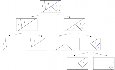
Fig. 2: Binary search tree construction illustration

Controller Complexity Reduction

The limiting factor to apply MPC is the amount of computational load involved. Explicit controller complexity can be reduced in a number of ways:

• Using move blocking – reduction of the degrees of freedom by fixing the input or its derivatives to be constant over several time-steps. MPT toolbox can handle a number of different move blocking strategies, but unfortunately these are only applicable to LTI systems with quadratic cost formulation
• The choice of penalties in the optimization problem will result in simpler solution (higher penalty on the control action results in fewer regions)
• Simplification of explicit solution. MPT toolbox is able to simplify explicit controllers by merging regions which contain the same control law.

One of the most useful methods in the optimal region merging (ORM) (Geyer et al., 2008). It should be noted that it is a frequent case in parametric MPC that there are multiple regions of the table in which the expression for u^* is the same. Thus the idea of ORM is to merge the regions which share the same expression for the optimizer into larger convex objects.

3.3 Reference Tracking MPC Problem

The basic MPC problem (13) and the corresponding mp-QP formulation (22) can be extended to reference tracking problem. The output, instead of being regulated to the origin, is required to either asymptotically converge to a constant reference value or follow a reference signal that may vary in time. In either case, the objective is to minimize the error between the system output y(t) and the reference signal y_ref ∈ R_p, which is given by the problem specifications and is a function of time. The general MPC formulation to treat the reference tracking problem is in the form:

(32a)

(32b)

(32c)

(32d)

(32e)

(32f)

(32g)

(32h)

Thus, the augmented state variable is in the form

(33)

where U = {Δu_k,…, Δu_k+N–1}, y_ref = { y_ref,k,…,y_ref,k+N}, and Δu∈R^m represent the control increments that act as correcting terms in the input to force the output to track the reference signal. The equation u_k = u_k–1 + Δuk corresponds to adding an integrator in the control loop. The reference tracking MPC (32) can be formulated into an mp-QP problem, just like the general MPC problem (13). By taking these extra parameters into account and repeating the procedure in Sections 3 and 3.2, we can transform the tracking problem (32) into

(34a)

(34b)

and into the mp-QP problem

(35a)

(35b)

where z = U + H^-1 F^T [x_k u_k-1 y_ref]^T and S = E + GH^-1 F^T. The solution of (35) U is a linear, piecewise affine function U(x_k, u_k–1, y_ref) of x_k, u_k–1, y_ref defined over a number of regions CR₀, where this solution is valid. The reference tracking MPC is implemented by applying the following control: u_k = u_k–1 + Δu_k(x_k, u_k–1, y_ref), where Δu_k(x_k, u_k–1, y_ref) is the first component of the vector U(x_k, u_k–1, y_ref).

4. MPC design via multi-parametric toolbox

The Multi-Parametric Toolbox (MPT) for Matlab developed by (Kvasnica et al., 2004) is a freely download-able tool that simplifies the design, analysis and deployment of optimal controllers for constrained linear, nonlinear and hybrid systems. Efficiency of the code is guaranteed by the extensive library of algorithms from the field of computational geometry and multi-parametric optimization. To calculate the explicit controller the MPT toolbox has interfaces to efficient commercial solvers such as for example CPLEX, NAG. It also provides a number of algorithms for computing with polytopic sets and the functions for their visualization. The visualization is helpful namely by analysis of designed MPC. We demonstrate the controller design capabilities of the toolbox with some examples in the following section.

4.1 Numerical Example 1: Discrete Dynamical System

Consider a discrete-time double integrator

which is subject to constraints −5 ≤ x ≤ 5, and −1 ≤ u ≤ 1. We consider the MPC problem with prediction horizon N = 7, quadratic norm and weighting matrices Q = diag(1, 0) and R = 1. For the double integrator example the mp-QP problem (22) has been solved using the MPT toolbox and constructed explicit representation of UN in the form of following PWA function was computed in just 2 seconds, defined over 7 polytopic regions, along with the piecewise quadratic (PWQ) function J^*(x):

The simulation results of the closed-loop system indicating the evolution of the states and the input for initial state [3, 1]^T are depicted on the Fig. 3.

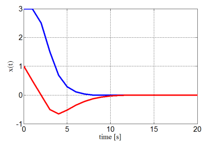
(a) Closed-loop state trajectories

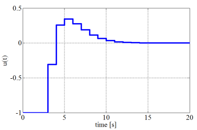
(b) Time response of the input signal

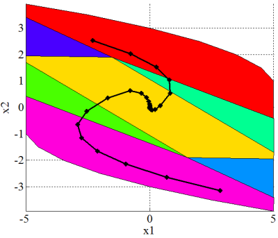
(c) Controller partition with the state trajectory for several initial states

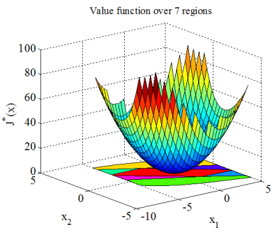
(d) PWQ optimal cost J^*(x)
Fig. 3: Results obtained from the example 1.

4.2 Numerical Example 2: Two-tank System Model

Consider now the system consisting of two liquid storage tanks placed one below the other. Liquid inflow to the upper tank is governed by a pump, throughput of which is to be controlled. The liquid in the first tank flows out through an opening to the lower tank. The state-space representation of the linearized system is in the form:

The control objective is to operate the pump such that the level in the lower tank reaches a given time varying reference signal, while respecting input and state constraints

The parameters of the MPC problem to be solved are Q = eye(2), _Qy = 10, R = 1 and N = 5. The control problem (20) has been augmented according to section 3.3 and solved parametrically via MPT toolbox, which provided the regions and the corresponding feedback laws. The result of the computation was in this case a lookup table consisting of 64 regions in the state-space. For comparison, an unconstrained quadratic MPC based on the same weighting matrices Q, R and Q_N solving the Riccati equation was constructed. This approach corresponds to the linear quadratic regulator (LQR). By using Matlab-Simulink we obtained the simulation results depicted in the Fig. 4. From the results it can be seen, that explicit MPC observes defined constraints whereas the LQR controller cannot deal with constraints and leads the input to the saturation.

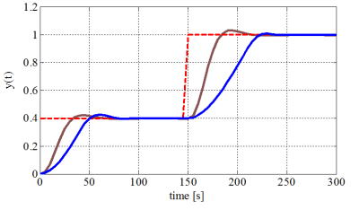
(a) Liquid level in the second tank (blue – explicit MPC, brown – LQR)

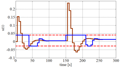
(b) Input flow
Fig. 4: Closed-loop simulation

5. Conclusion

Conventional model predictive control (MPC) implementation requires at each sampling time the solution of an open-loop optimal control problem with the current state as the initial condition of the optimization. Formulating the MPC problem as a multi-parametric programming problem, the online optimization effort can be moved offline and the optimal control law defined as a piecewise affine (PWA) function with dependence on the current state. The domain where the PWA function is defined corresponds to the feasible set which is partitioned into convex regions.

The online computation reduces to simple evaluations of a PWA function, allowing implementations on simple hardware and systems with fast sampling rates. Furthermore, the closed form of the MPC solutions allows offline analysis of the performance, providing additional insight of the controller behavior. In this paper a general framework for multiparametric programming and explicit MPC control design was presented and applied in several examples.

6. Acknowledgement

References

1. A. Bemporad and M. Morari. Control of systems integrating logic, dynamics, and constraints. Automatica, 35, 407–427, 1999.
2. A. Bemporad, M. Morari, V. Dua, and E.N. Pistikopoulos. The explicit solution of model predictive control via multiparametric quadratic programming. American Control Conference, 2000
3. F. Borrelli, M. Baotic, A. Bemporad, and M. Morari. Efficient On-Line Computation of Explicit Model Predictive Control. Technical report, August 2001
4. E.G. Gilbert and K. Tin Tan. Linear systems with state and control constraints: the theory and applications of maximal output admissible sets. IEEE Trans. Automatic Control, 36(9):1008–1020, 1991
5. P. Grieder and M. Morari. Complexity reduction of receding horizon control. Proceedings of 42nd IEEE Conference on Decision and Control, 3, 2003
6. T. Geyer, F. Torrisi, M. MORARI. Optimal complexity reduction of polyhedral piecewise affine systems. Automatica, 44, 7, 2008
7. M. Kvasnica, P. Grieder, and M. Baotic. Multi-Parametric Toolbox (MPT), 2004
8. D.Q. Mayne, J.B. Rawlings, C.V. Rao, and P.O.M. Scokaert. Constrained model predictive control: Stability and optimality. Automatica, 36(6):789-814, 2000
9. J.B. Rawlings and K.R. Muske. The stability of constrained receding-horizon control. IEEE Trans. Automatic Control, 38:1512–1516, 1993
10. P. Tøndel, T.A. Johansen, and A. Bemporad. Evaluation of piecewise affine control via binary search tree. Automatica, 39(5):945-950, 2003
11. F.D. Torrisi, A. Bemporad, G. Bertini, P. Hertach, D. Jost, D. Mignone. Hysdel 2.0.5 – User Manual, 2002

---

Institute of Control and Industrial Informatics, Faculty of Electrical Engineering and Information Technology, Slovak University of Technology in Bratislava