This work concentrates on performance evaluation of bandwidth allocation methods in MPLS-TE networks supporting Diffserv (DS-TE networks). Bandwidth allocation in such networks is executed by Bandwidth Constraint Models (BCM). We provide a brief summarization of BCMs. Afterwards we focus on the three standardized BCMs which are compared based on the achieved Quality of Service (QoS) characteristics. We used Network Simulator 2 (NS-2) environment for our simulations.

1. Introduction

The variety of today’s multimedia traffic calls for an effective mechanism to ensure desired Quality of Service (QoS) parameters (Chromy, et al., 2013). Delay, jitter and loss values should be evaluated to fulfil the traffic’s needs (Halas, et. al, 2012). DiffServ-aware MPLS-TE (DS-TE) networks introduces concept of combining properties of MPLS-TE and DiffServ. MPLS-TE provides connection-oriented approach in IP networks. It creates end-to-end paths (LSPs) where it can guarantee bandwidth and with traffic engineering it can truly optimize network’s resources. The problem of original concept of MPLS-TE was the unawareness of the actual traffic it was carrying.

DiffServ model is implemented to make it aware of the traffic class. Previously not actually used Exp bits in MPLS header are replaced by CoS (Class of Service) bits which are designated to carry PHB information. There are two approaches depending on how many traffic classes are to be supported in the network. The networks with up to 8 classes use E-LSP (Exp-inferred LSP) where only CoS bits are used to carry PHB information. Networks where more than 8 classes are required should use L-LSP (Label-inferred LSP) where label itself is used to carry PHB information (scheduling behaviour) and CoS bits are used to distinguish drop priority.

The process of bandwidth allocation in such networks is executed by Bandwidth Constraint (BC) models, which introduce the logic of how the available bandwidth is to be divided between the traffic classes. The article is divided as follows. In chapter 2 we provide the survey of BC models. In chapter 3 we present our simulation model with simulation scenario. Chapter 4 provides the initial results of our simulations. In chapter 5 we tried to tune up the models and we present the final results. We conclude the article in chapter 6.

2. Bandwidth constraint models

In DS-TE networks, the bandwidth allocation between various classes is determined from the relation between Class Type (CT) and Bandwidth Constraint (BC) (Adami, et al., 2008).
CT is a group of traffic trunks based on their QoS values so that they share the same bandwidth reservation, and a single class-type can represent one or more classes. CT is used for bandwidth allocation, constraint routing and admission control. Bandwidth Constraint (BC) is a limit on the percentage of a links bandwidth that a particular class-type can use. BC models determine how the bandwidth of the link is divided between various classes by defining the relation between CT and BC.

2.1 Maximum Allocation Model (MAM)

MAM (Le Faucher and Lai, 2005) is the first and the simplest BC model which maps one BC into one CT. Thus the bandwidth of every CT is separated from other CTs. Fig. 1 shows how MAM works (for simplification only 3 CTs are shown).

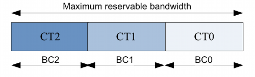
Fig. 1. MAM.

Advantage of MAM is the ability to guarantee the bandwidth for every CT within the range of BC. The drawback of this model is low utilization due to the fact that CTs cannot use the unused bandwidth of other CTs.

2.2 Maximum Allocation with Reservation Model (MAR)

because it also allocates bandwidth for every CT. The difference is that CTs can exceed this value if there is no congestion. If the congestion happens the CTs revert to their original allocated bandwidth. The new request B_new from CT_i on link k is accepted if the following rules are met:

• LSPs with high and normal priority CT_i:
  • If B_res,i,k ≤ BCc,k then accept if Bnew ≤ Bunres,k
  • If B_res,i,k>BC_c,k then accept if B_new ≤ B_unres,k – B_tresh
• LSPs with low priority CT_i:
  • Accept if B_new ≤ B_unres,k – B_tresh

Where B_tresh represents bandwidth on link k which can be accessed if given CT_i has actually reserved bandwidth B_res,i,k under the value of allocated bandwidth constraint BC_i,k. If B_res,i,k exceeds BC_i,k then B_tresh cannot be accessed. Fig.3 shows bandwidth division in MAR.

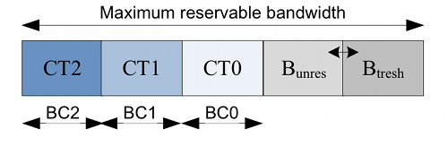
Fig. 2. MAR.

2.3 The Russian Dolls Model (RDM)

RDM (Le Faucher, 2005) differs from MAM or MAR by allowing CTs to share the bandwidth between each other. CT7 represents the traffic with the strictest QoS demands and CT0 represents best effort traffic. BC7 represents the bandwidth dedicated just for CT7, BC6 is dedicated for CT7 and CT6, BC5 is dedicated for CT7, CT6 and CT5, and so on. This way the bandwidth´s utilization is more effective but there is no guaranteed bandwidth for lower priority classes. The model is represented in Fig. 2 (only 3 CTs are shown for simplicity).

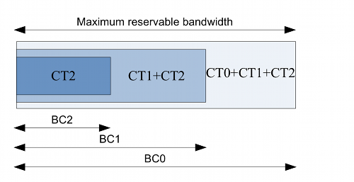
Fig. 3. RDM.

2.4 Other BC models

Generalized RDM (G-RDM)

G-RDM (Adami, et al., 2007) uses the best from MAM and RDM. It guarantees a predefined amount of bandwidth for each CT and at the same time allows the bandwidth sharing. There are defined two pools for every CT_i. The private pool n_i is the guaranteed bandwidth for the CT_i and the common pool m_i represents the bandwidth that can be shared between the classes.

Blocking Constraint Model (BCM)

The aim of BCM (Goldberg, et al., 2007) is to give priority to those LSPs for which the considered link is the last link on the path.BCM behaves exactly the same way as MAM except for the last link where it upgrades the pre-emption permission on the LSP with following effect:

• High priority class on last link (HP-LL) can pre-empt High priority class (HP), Medium priority class (MP), Low priority class (LP), MP on last Link (MP-LL) and LP on Last Link (LP-LL).
• MP-LL can preempt HP, MP, LP, LP-LL.
• LP-LL can preempt HP, MP, LP.

Max-Min model

Max-Min (Shan and Yang, 2007) defines minimum and maximum BC for each CT. The minimum bandwidth is guaranteed for every CT. Max-min model uses “Use it or lend it” strategy so if the CT doesn´t use its maximum bandwidth it can lend it to those CTs that could use it. If the demands of the CT rise, it will pre-empt those CTs that it lent the bandwidth to.

Adapt-RDM

Adapt-RDM (Pinto Neto and Martins, 2008) tries to improve RDM in a situation when BC limit for given CT is exceeded. The approach is based on a centralized management operation in which a management entity has the knowledge about the configured and established LSPs in the network. For each CT with lower priority than the CT corresponding to the new request, it is verified if bandwidth limits were exceeded. In affirmative cases, the bandwidth reduction function is invoked with a configurable parameter defined by the network manager.

AllocTC-Sharing Model

AllocTC-Sharing model (Reale, et al., 2011) adopts two different styles for bandwidth sharing concomitantly.
The “high-to-low” bandwidth allocation style is the classical alternative used in RDM. In this case, the non-used bandwidth reserved for high priority classes may be temporarily allocated to low priority classes. The “low-to-high” bandwidth allocation style innovates by allowing high priority classes temporarily allocate non-used bandwidth primarily reserved for low priority classes.

3. Simulation model

We performed our simulations in The Network Simulator 2 (NS-2) with MTENS patch extension. There are three traffic classes representing voice, video and data in the simulated network. The network consists of three traffic sources and three traffic sinks, one for every class. Between them there is a bottleneck MPLS link where the particular BC model is implemented (see Fig.4).

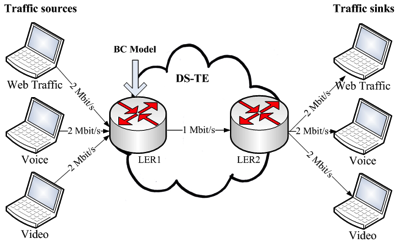
Fig. 4. Simulation Model.

We compare MAM, RDM and MAR models based on their ability to provide chosen QoS parameters. Each traffic source generates multiple traffic flows with various characteristics common for all the models. See Table I for detailed description of traffic flows.

Table I. – Traffic description

Flow ID	Traffic Source	Packet Size [B]	Rate [kbits/s]	Start [s]	Stop [s]
1	Web	600	350	2	16
2	Web	600	350	3	17
3	Voice	242	96,8	1	14
4	Voice	242	96,8	4	10
5	Video	655	261,8	5	13
6	Video	655	261,8	11	18

The web traffic is simulated with traffic generator with exponential distribution with On/Off intervals set to 500ms/500ms. The voice traffic is simulated in G.711 manner so constant bit rate generator is applied. The packets are sent every 20 ms. The bit rate 96,8 kbit/s is computed as G.711’s 64 kbit/s with all the necessary headers (RTP, UDP, IP, MPLS and Ethernet) resulting in 242 B header.

The video traffic is also simulated using constant bit rate where the packets are sent every 20 ms. The proposed 261,8 kbits/s is reached using DivX codec of a 40 minutes long video with size of 100 MB with audio bit rate of 112 kbit/s. As with the voice traffic we included all the necessary headers leading to the packets of 655 B.

4. Results

First we present the simulation results of each particular BC model. Then we compare the models based on the chosen criteria. The models are sensitive to parameter setup (bandwidth constraints for particular CT) so it is necessary to find an optimal value.

4.1 MAM

We chose the following division of bandwidth constraints between the CTs:

• BC₀ = 350 kbit/s (web traffic)
• BC₁ = 150 kbit/s (voice traffic)
• BC₂ = 500 kbit/s (video traffic)

The resulting throughput of the flows can be observed in Fig. 5.

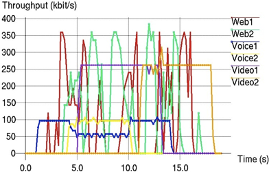
Fig. 5. Flows’ throughput using MAM.

As you can see Voice1 traffic starts to transmit at its given rate of 96,8 kbit/s. The next flow Web1 has no impact on it because in MAM allocated bandwidths of the CTs are isolated. Web1’s rate is decreased when Web2 flow starts to transmit because they together want to transmit at the maximum rate 700 kbit/s but their bandwidth constraint limits them only to 350 kbit/s. Similar situation happens with the voice when Voice2 flow starts to transmit. The voice flows want to transmit at 193,6 kbit/s rate but their BC limits them only to 150 kbit/s. Due to the BCs’ separation, the video traffic has no impact on web and voice traffic. Rate adjustment happens when Video1 and Video2 flows transmit at the same time (523,6 kbit/s desired bandwidth with BC=500 kbit/s).

4.2 RDM

We chose the same bandwidth constraint division as in MAM’s simulation. The resulting throughput of flows can be observed in Fig.6.

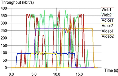
Fig. 6. Flows’ throughput using RDM.

RDM allows lower priority CTs to borrow unused bandwidth from higher priority CTs. The situation for Video traffic is unchanged because this CT is not allowed to borrow bandwidth from lower priority CTs. Voice traffic is transmitted without losses because it borrows bandwidth from Video traffic during the time both Voice flows are transmitting. Web traffic borrows bandwidth from both Video and Voice. But even so there are periods when the borrowed bandwidth does not fully satisfy its needs For example in 5 s – 10 s interval the requested bandwidth of Web traffic is 600 kbit/s and available bandwidth is 444,6 kbit/s (BC₀ = 350 kbit/s + borrowed bandwidth 94,6 kbit/s).

4.3 MAR

For this particular BC model we chose the following BC division:

• BC₀ = 200 kbit/s
• BC₁ = 150 kbit/s
• BC₂ = 450 kbit/s
• B_tresh = 200 kbit/s

The resulting throughput of the flows can be observed in Fig. 7.

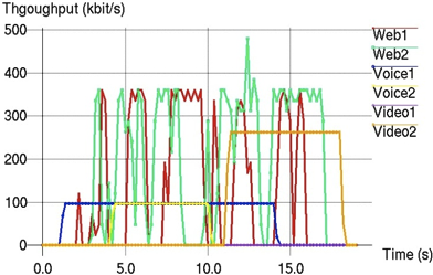
Fig. 7. Flows’ throughput using MAR.

MAR admits the flows according to the conditions mentioned in chapter 2.2. Voice1 and Web1 flows fulfil the conditions B_res,i,k ≤ BC_c,k and B_new ≤ B_unres,k and are therefore admitted. Web2 flow does not fulfil the first condition because Web1 exceeded BC0 but it fulfils the following condition that B_new ≤ B_unres,k – B_tresh (350 kbit/s ≤ 608,2 kbit/s – 200 kbit/s). Voice2 fulfils both conditions so it is admitted. When Video1 flow wants to transmit it fulfils the first condition but it is not admitted because it fails the subsequent condition B_new > B_unres,k (261,8 kbit/s > 212,7 kbit/s). The Video2 flow can be admitted because it arrives at the time when Voice2 flow no longer transmits so Bunres,k is increased.

4.4 BCMs Comparison

We compared the three models according to their ability to provide QoS. BCMs were compared based on delay, jitter, loss and network utilization. First the flows were compared based on their end-to-end delay and jitter values in Tables II, III and IV.

Table II. – MAM QOS comparison

Flow	Delay			Jitter
	Avg. [ms]	Min. [ms]	Max. [ms]	Avg. [ms]	Max. [ms]
Web1	75.32	39.6	120	5.757	59.31
Web2	64.6	39.6	115.5	6.033	66.76
Voice1	54.14	33.88	100.76	3.567	20.39
Voice2	61.68	33.87	102.4	4.995	18.1
Video1	46.05	40.48	93.05	1.258	14.75
Video2	45.84	40.48	88.26	1.076	14.78

Video traffic has the lowest average delay because the loss of this traffic is the lowest so there were the lowest number of packets waiting and being dropped from the buffer. The network fulfils the ITU recommendation that voice should be below the 150 ms value where the maximum delay of voice is 102,4 ms.

Table III. – RDM QOS comparison

Flow	Delay			Jitter
	Avg. [ms]	Min. [ms]	Max. [ms]	Avg. [ms]	Max. [ms]
Web1	50.45	39.6	90.3	2.866	42.4
Web2	49.8	39.6	86.79	2.577	29.68
Voice1	37.07	33.87	49.59	2.56	15.72
Voice2	35.8	33.87	43.84	2.535	9.873
Video1	46.62	40.48	93.05	1.689	14.75
Video2	46.08	40.48	88.26	1.425	14.776

For RDM, the delay and jitter values are different compared to MAM (See Table III). Web and Voice traffic does not spend as much time in buffer so the resulting values are smaller. Video traffic has practically the same values because for this CT nothing has changed.

Table IV. – MAR QOS comparison

Flow	Delay			Jitter
	Avg. [ms]	Min. [ms]	Max. [ms]	Avg. [ms]	Max. [ms]
Web1	45.32	39.6	116.5	1.627	68.8
Web2	44.22	110	86.79	1.68	8.915
Voice1	35.91	33.87	43.89	1.676	9.788
Voice2	34.79	33.87	38.66	1.506	4.783
Video1	x	x	x	x	x
Video2	41.36	40.48	45.27	1.166	4.786

Because MAR did not let one flow (Video1) in the network the utilization dropped and so the buffers are less loaded resulting in the smaller delay and jitter values compared to MAM and RDM (See Table IV). To better illustrate delay and jitter comparison we add Figures 8 and 9 representing average delay and jitter comparison of the BCMs.

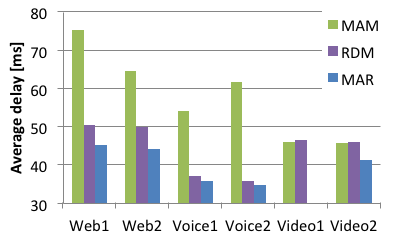
Fig. 8a. Comparison of BCMs based on flows’ average delay.

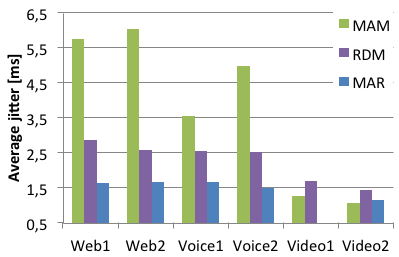
Fig. 8b. Comparison of BCMs based on flows’ average jitter.

The Table V represents the loss comparison. The overall, web, voice and video loss rates are compared for each BCM.

Table V. – Loss comparison

BCM	Loss [%]	Loss (web) [%]	Loss (voice) [%]	Loss (video) [%]
MAM	13,06	22,25	12,58	0,39
RDM	1,59	3,91	0	0,39
MAR	0	0	0	0

As could be expected, MAM provides the worst properties in loss comparison. This is due the fact that it does not allow bandwidth borrowing as RDM where overall loss is much smaller. Video loss is unchanged in RDM because the highest priority class does not borrow bandwidth from lower priority classes. MAR model seems to have zero loss in all categories. But this is achieved by not allowing Video1 flow into the network. As can be seen in Table VI, MAR has the lowest utilization and also the lowest number of generated packets among the BC models. MAM and RDM generate the same amount of packets but because of higher loss rate in MAM and bandwidth sharing in RDM, RDM model utilizes the network in best way.

Table VI. – Network utilization comparison

BCM	Utilization [%]	Packets generated	Bytes generated
MAM	55,72	2711	1357128
RDM	62,65	2711	1357128
MAR	54,11	2461	1149899

5. Tuning up the models

In this chapter we try to tune up the BC models. We use oversubscription for MAM and RDM. The oversubscription enables that the sum of allocated bandwidth constraints is higher than the maximum reservable bandwidth. For MAR model we use various values of B_tresh to stress its impact to various traffic types.

5.1 Implementing oversubscription for MAM and RDM

We chose the following division of bandwidth constraints between the CTs for MAM:

• BC₀ = 700 kbit/s (web traffic)
• BC₁ = 200 kbit/s (voice traffic)
• BC₂ = 550 kbit/s (video traffic)

The values were chosen so that BCs could accommodate both traffic flows from its traffic type. For example BC₂’s value of 550 kbit/s is able to accommodate both video flows (523,6 kbit/s). We only increased BC₂ value for RDM model because voice traffic is already transmitted without losses and increasing web’s BC₀ would have no sense because this traffic class can borrow any unused bandwidth of higher priority classes. The BC division si as following:

• BC₀ = 350 kbit/s (web traffic)
• BC₁ = 150 kbit/s (voice traffic)
• BC₂ = 550 kbit/s (video traffic)

The resulting throughput graph is depicted in Figure 9. We also add loss rates comparison in Table VII.

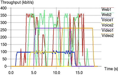
Fig. 9. Flows’ throughput using MAM/RDM with oversubscription

Table VII. – Loss comparison of oversubscribed MAM and RDM

BCM	Loss [%]	Loss (web) [%]	Loss (voice) [%]	Loss (video) [%]
MAM	1,51	3,91	0	0
RDM	1,51	3,91	0	0

As you can see by implementing oversubscription MAM achieved the same results as RDM. This is because web traffic is able to use bandwidth that is currently unused by higher classes (video) so in a way it borrows the bandwidth from higher classes just like in RDM model. But implementing oversubscription can have its drawbacks. Setting BCs too high diminishes the main aim of MAM which is guaranteeing the bandwidth for each class within its BC. If we set BC₁ and BC₂ too high and voice and video’s requirements were too high, the web traffic would have no spare bandwidth to use resulting in very high losses and unusable service.

5.2 Setting the proper threshold value for MAR

Results in chapter 4 showed that MAR rejected highest priority Video1 flow. To give higher priority flows preferable treatment over web traffic we set BC₀ to 0 kbit/s. This way web traffic is considered best effort and is admitted only if currently unreserved bandwidth minus threshold bandwidth can fulfils their requirements. So the BC division is as following:

• BC₀ = 0 kbit/s (web traffic)
• BC₁ = 150 kbit/s (voice traffic)
• BC₂ = 450 kbit/s (video traffic)

The higher we set the B_tresh value the more we penalize best effort traffic (web) and flows which exceed their BC. When the network is not congested B_tresh value should be set as low as possible so that best effort traffic is not rejected and there are enough resources in the network. In congested network as is our case we should increase B_tresh so that we decrease the probability that lower priority flows are responsible for rejecting the higher priority flows. The resulting admittance of the flows is depicted in Table VIII.

Table VIII. – Impact of various B_tresh values on flows’ admission

Flow	Btresh [kbit/s]
	0 – 300	350 – 550	600 – 1000
Web1	admitted	admitted	rejected
Web2	admitted	rejected	rejected
Voice1	admitted	admitted	admitted
Voice2	admitted	admitted	admitted
Video1	rejected	admitted	admitted
Video2	admitted	admitted	admitted

The table shows that low values of B_tresh up to 300 kbit/s result in rejecting highest priority Video1 flow. Setting the values in 350 – 550 kbit/s interval resulted in rejecting Web2 flow instead of Video1 flow. This is because B_unres,k – B_tresh is lower than Web2’s requirements (350 kbit/s). And because this flow was rejected there was sufficient bandwidth for Video1. As you can see setting B_tresh too high resulted in unnecessary rejection of Web1 flow which could otherwise be admitted.

5.2 BCMs comparison

Here we compare BCMs again based on the achieved delay (Fig. 10) and jitter (Fig. 11) values.

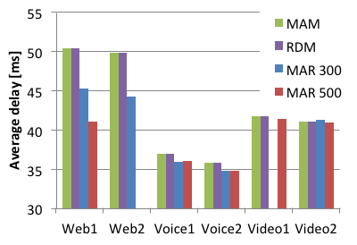
Fig. 10. Comparison of tuned up BCMs based on flows’ average delay.

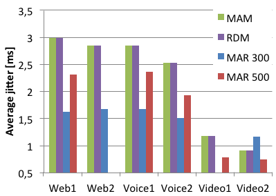
Fig. 11. Comparison of tuned up BCMs based on flows’ average jitter.

average jitter.
As you can see oversubscribed MAM and RDM achieved the same performance. MAR overall achieved the lowest delay and jitter values where MAR 300 implements B_tresh = 300 kbit/s and MAR 500 implements B_tresh = 500 kbit/s.

6. Conclusion

We compared the standardized Bandwidth Constraint Models based on numerous properties. MAM is the simplest model but behaves very conservative. It isolates each CT which results in the worst properties of the models. RDM utilizes best the network resources with better QoS parameters than in MAM. RDM mainly profits from the ability to share bandwidth between CTs. Its drawback is inability of higher priority classes to borrow bandwidth from lower priority classes. Implementing oversubscription can further tune up MAM or RDM by letting classes to use previously unused bandwidth of classes with lower requirements than its BC. But implementing this mechanism diminishes BC isolation and the bandwidth guarantees for the classes. If higher priority classes had very high requirements the lower priority classes could be completely starved. So it must be taken into consideration if it is preferable to maintain strict bandwidth constraint separation or to allow oversubscription which could starve lower priority classes so that higher priority classes could be transmitted with lower loss and delay.

MAR offers a different approach utilizing bandwidth threshold parameter which influences the degree that the higher priority traffic is prioritized over lower priority. We showed that too low values can cause higher priority flows not to be admitted because of lower priority flows. On the other hand, too high values of the treshold can cause unnecessary rejection of low priority flows. The given standardized BC models have their weaknesses which are addressed by proposing new BC models (as mentioned in chapter 2.4).

Acknowledgment

This work is a part of research activities conducted at Slovak University of Technology Bratislava, Faculty of Electrical Engineering and Information Technology, Institute of Telecommunications, within the scope of the project VEGA No. 1/0106/11 “Analysis and proposal for advanced optical access networks in the NGN converged infrastructure utilizing fixed transmission media for supporting multimedia services” and „Support of Center of Excellence for SMART Technologies, Systems and Services II., ITMS 26240120029, co-funded by the ERDF“.

References

1. Adami,D., C. Callegari, S. Giordano, M. Pagano (2008). A New NS2 Simulation Module for Bandwidth Constraints Models in DS-TE Networks. In: ICC 2008, pp. 251-255.
2. Adami,D., C. Callegari, S. Giordano, M. Pagano and M. Toninelli (2007). G-RDM: A New Bandwidth Constraints Model for DS-TE networks. In: GLOBECOM 2007, pp. 2472-2476.
3. Ash, J. (2005). IETF RFC 4126: Max Allocation with Reservation Bandwidth Constraints Model for Diffserv-aware MPLS Traffic Engineering & Performance Comparisons.
4. Goldberg,J. B., S. Dasgupta, J. Cavalcante de Oliveira (2006). Bandwidth Constraint Models: A Performance Study with Preemption on Link Failures. In: GLOBECOM 2006, pp. 1-5.
5. Halas, M., A. Kovac, M. Orgon, I. Bestak (2012). Computationally Efficient E-Model Improvement of MOS Estimate Including Jitter and Buffer Losses. In: Telecommunications and Signal Processing TSP-2012, pp. 86-90, ISBN 978-1-4673-1116-8.
6. Chromy, E., M. Jadron and T. Behul (2013): Admission Control Methods in IP Networks. In Advances in Multimedia, vol. 2013, Article ID 918930, 7 pages, 2013, ISSN: 1687-5680 (Print), ISSN: 1687-5699 (Online), doi: 10.1155/2013/918930.
7. Le Faucheur, F. and W. Lai (2005). IETF RFC 4125: Maximum Allocation Bandwidth Constraints Model for Diffserv-aware MPLS Traffic Engineering.
8. Le Faucheur, F. (2005). IETF RFC 4127: Russian Dolls Bandwidth Constraints Model for Diffserv-aware MPLS Traffic Engineering.
9. Pinto Neto, W. and J. Martins (2008). Adapt-RDM – A Bandwidth Management Algorithm suitable for DiffServ Services Aware Traffic Engineering. In: IEEE/IFIP Network Operations & Management Symposium.
10. Reale,R. F., W. da C. P. Neto and J. S. B. Martins (2011). AllocTC-sharing: A new bandwidth allocation model for DS-TE networks. In: LANOMS 2011, pp. 1-4.
11. Shan, T. and O. W. W. Yang (2007). Bandwidth Management for Supporting Differentiated Service Aware Traffic Engineering. In: IEEE Transactions On Parallel And Distributed Systems, vol. 18, no.9, pp. 1320-1331.

---

Coauthor of this paper is M. Medvecký, Institute of Telecommunications, Faculty of Electrical Engineering and Information Technology, Slovak University of Technology in Bratislava