Virtual hydraulic system realized on PLC
27. August, 2014, Autor článku: Körösi Ladislav, Elektrotechnika
Ročník 7, číslo 8  Pridať príspevok
![]() In this paper description of virtual hydraulic system realized on Programmable Logic Controller (PLC) is described. The aim of this paper is to present the basic properties of hydraulic system and show the possibility of its simulation directly in PLC system without need of using of software and hardware.
In this paper description of virtual hydraulic system realized on Programmable Logic Controller (PLC) is described. The aim of this paper is to present the basic properties of hydraulic system and show the possibility of its simulation directly in PLC system without need of using of software and hardware.
1. Introduction
Recently, expansion of different software techniques for modelling of real systems is observed. These techniques make simply analyses of properties of given nonlinear process. On the basis of these analyses could be with properly specific methods also the parameters of controllers designed. Then the model can be controlled in real time. These techniques are finance less than the experiments on real system, which many times can’t be realized (e.g. by reason of continuous regulation). Firstly the description of hydraulic system with open-top tank (top of reservoir open to the atmosphere) is presented in detail. In the next section the design and realization of the virtual hydraulic system are introduced. The last section offers the simulation results of all analyses of designed model.
2. Hydraulic System
Consider an open tank with the inlet flow rate M1 and output flow rate M2, where the atmospheric pressure acts on water level (Fig. 1)
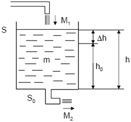
Fig. 1. Hydraulic system with free outlet (S – water surface area [m2], S0 – cross sectional area of the hole [m2], m – mass of the liquid in the tank [kg], Mi -mass flow of fluid at the inlet and outlet of the tank [kg.s-1], h – water level [m])
The hydraulic model is based on the law of conservation of matter:
 |
(1) |
 |
(2) |
Where V is the volume of liquid in the tank [m3], ρ is the density of the liquid [kg.m-3], Qi is the volumetric liquid flow rate at the inlet and outlet of the tank [m3.s-1]. We consider S=const.
 |
(3) |
For water flow rate:
 |
(4) |
Where g is the gravitational acceleration = 9.81 ms-2. Then
 |
(5) |
Where μ is the coefficient of outflow ϵ (0, 1), for water µ = 0.63, S2 is the cross beam of the outflowing fluid [m2].
Virtual model description
The following relation describes the difference of the water level in the tank.
") |
(6) |
Virtual model was implemented in Unity Pro using Structured text programming language in discrete form. The parameters of the virtual model were: S = 1m2, S0 = 0.01m2, Ts = 1s, where Ts is the sampling time.
3. Design and Realization of Virtual Model
Virtual model of hydraulic system has been designed and implemented in system Unity Pro XL in 7.0 from Schneider Electric. It is programmable and configuration software for M340, Premium and Quantum PAC systems. Main selection criterion is possibility of simply implementation of language code, structured text with simulation application of created project in built PLC emulator. There is also possibility of connecting real and simulated visualization to emulator. Model of hydraulic system was designed as derived function block (DFB). User’s DFB includes data (in PLC systems – data blocks DB) and also algorithms. Program is in PLC memory only ones, therefore by using more DFB instances, we notice saving of memory and clarity of designing program too. Parts of algorithm can be created in more sections; each of sections can have different program language.
Inputs of virtual model DFB of hydraulic system are shown in Fig. 2. Input Enable is used to enable or denied of virtual model simulation. Input Flow is input flow into tank [m3/h]. Second input Flow_fault, analogous to Flow, is input flow into tank and used to input noise simulation. This flow is not measurable, therefore is separated from input Flow.

Fig. 2 Inputs of virtual model DFB of hydraulic system
List of outputs of virtual model DFB of hydraulic system are given in Fig. 3. Signal Level_filtered determines filtered high of simulated high of level. Signal Level is noise signal of Level_filtered, which can be used to testing of noise sensitive etc. Signal Tic has value TRUE each sample time, which is defined by Timer (see local variables of PLC).

Fig. 3 List of the outputs of virtual model DFB of hydraulic system
List of global variables, which can be change using visualization or animation table etc., is in Fig. 4. Variables Flow_lo_value and Flow_hi_value define the constraint of the input flow what means from 0% to 100% of valve open or speeds of pump, which can control the input flow. Upper and lower bounds of flow rate (Flow_close_rate_value, Flow_open_rate_value) were considered to make the model closer to reality . These signals manipulate with maximum values of increase of opening and closing valve, which means opening of valve from 0% to 100% not incrementally, but linear. Minimal and maximal levels in tank are defined by variables Level_lo_value and Level_hi_value. The parameters of tank are S – surface of tank and S0 – outlet surface. Sample time (update for value change) is T. Range of simulation noise, which is added to the calculated height of level, is from Noise_lo_value to Noise_hi_value. Signal Noise_init serves as constrained initialization of initial values of random noise.
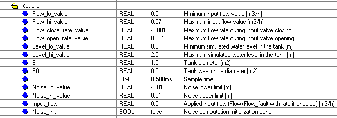
Fig. 4 Global variables of the virtual hydraulic system
Private variables (Fig. 5) are so called local variables (tags), which couldn’t be monitored by software, visualization etc. They are used for temporary storage of values which are not so important for monitoring or for parameterization. For example tags Noise_k and Noise_q are used for linear transformation of noise according to equation Noise_value_REAL := (Noise_k * DINT_TO_REAL(Noise_value_DINT) + Noise_q); and for conversion from DINT to REAL data type.
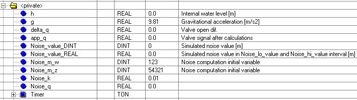
Fig. 5 Local variables of the virtual hydraulic system
In Fig. 6 two sections are presented. First section noise_simulation is used to simulate the noise for water level measurement which is based on the next expression [1]:
m_w =
/* must not be zero, nor 0x464fffff */
m_z =
/* must not be zero, nor 0x9068ffff */
uint get_random()
{
m_z = 36969 * (m_z & 65535) + (m_z >> 16);
m_w = 18000 * (m_w & 65535) + (m_w >> 16);
return (m_z << 16) + m_w;
/* 32-bit result */
}
There are two modifications. The first provides random initialization of m_w and m_z tags depending on the system time, actual cycle length etc. The second one returns the absolute value of the last equation. Section level_simulation contains all expressions mentioned in the beginning of the proposed paper implemented with simulation of variable saturation, rate change etc. Both sections were programed in Structured Text (ST) programing language.
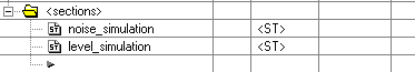
Fig. 6 List of DFB sections of the simulated model
4. Verification of properties of the virtual model
Input-output characteristics of the virtual model with S = 1m2, s0 = 0,01m2 parameters are in Fig. 7. The first characteristic (red color) was measured without level saturation. Second characteristic (black color) was measured with maximal level 2m.
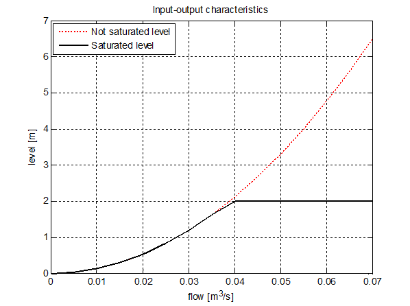
Fig. 7 Input-Output characteristics of the virtual hydraulic system
Comparison of time responses of the desired flow and measured flow which was limited to maximum rate 0,001 m3/h for all directions (opening and closing) is shown in Fig. 8. Without simulation of the flow rate saturation both flow values (desired and measured) would be the same.
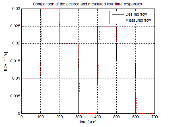
Fig. 8 Comparison of time responses of the desired and the measured input flows
Comparison of the filtered and not filtered tank level time responses is shown in Fig. 9. Noise level depends on the defined interval (Noise_lo_level, Noise_hi_level) which was in our simulations ±0,01m.
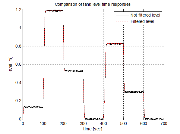
Fig. 9 Comparison of the filtered and not filtered tank level time responses
Comparison of the filtered and not filtered tank level time responses for different input flows (u) with maximum input flow rate is shown in Fig. 10. In figure three step responses are compared for the following input flows: 0,01, 0,02 a 0,03 m3/h.
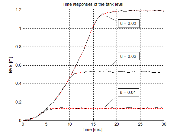
Fig. 10 Comparison of the filtered and not filtered tank level time responses for different input flows (u) with maximum input flow rate 0.001 m3.s-1
Examples of time responses of the water level without input flow rate limitation on the tank inlet is shown in Fig. 11. In Fig. 11 three characteristics are compared in the same ways as in Fig. 10 (input flows: 0,01, 0,02 a 0,03 m3/h). Comparing results in Fig. 10 with Fig. 11 could lead to different model order in process of identification therefore the simulated model depends on the parameter set.
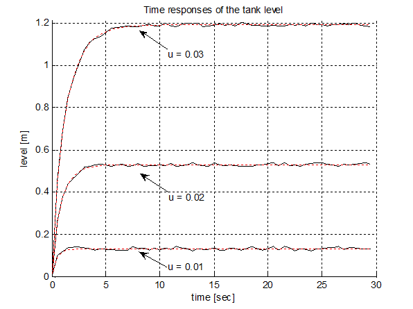
Fig. 11 Comparison of the filtered and not filtered tank level time responses for different input flows (u) without maximum input flow rate limitation
To verify the performance of the proposed PID controllers, simulation of disturbance is often used. Time response of the tank level for constant input flow depending on the variable input flow disturbance is shown in Fig. 12. Time response of the input flow disturbance is in Fig. 13.
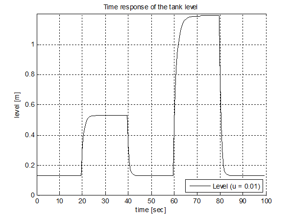
Fig. 12 Time response of the tank level for constant input flow (u = 0.01 m3.s-1) and variable input flow disturbance

Fig. 13 Time response of the input flow disturbance
Disturbance simulations with the output gauge diameter change (simulation of the valve opening or closing) are in Fig. 14 and 15. Time response of the tank level depending on change of the output gauge diameter is in Fig. 14 and time response of the disturbance simulation is in Fig. 15.
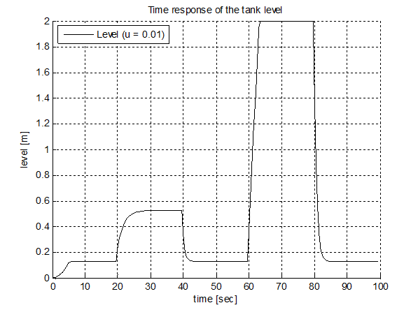
Fig. 14 Time response of the tank level depending on change of the output gauge diameter
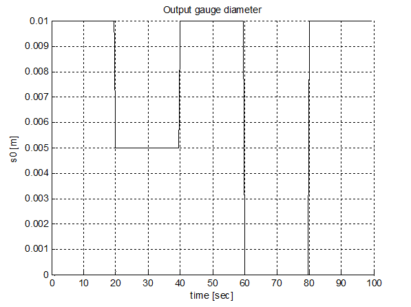
Fig. 15 Changes of the output gauge diameter for disturbance simulation
Detailed view of the simulated noise which was added to the tank level is shown in Fig. 16. Noise histograms are shown in Fig. 17 and 18. The generated random noise has normal distribution.
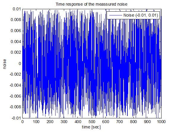
Fig. 16 Time response of the measured noise
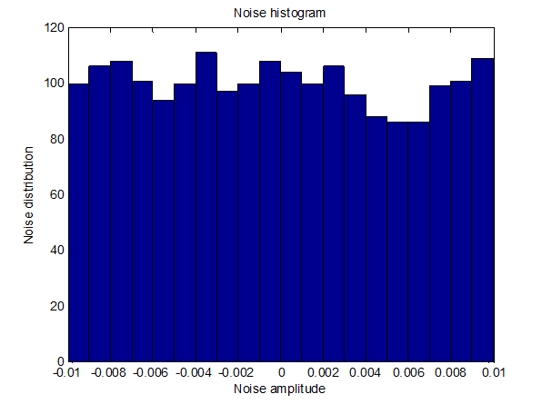
Fig. 17 Noise histogram
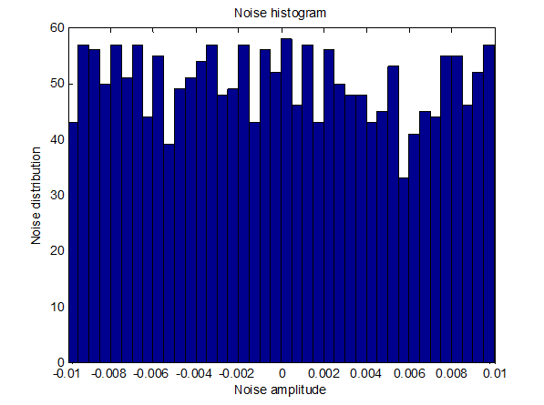
Fig. 18 Detailed noise histogram
5. Conclusion
In this paper the design, implementation and verification of the hydraulic system’s model was presented. In contrast to other approaches, where the model is realized using software tools, it is necessary to ensure the communication between the PLC and the model; the hydraulic system was implemented directly in the PLC. In the designed model signal limitations were considered which mimics the real process behavior. This application will be used in pedagogic process and for research tasks.
Acknowledgement
This paper has been supported by the Slovak Scientific Grant Agency, Grant No. 1/2256/12 and Grant No. 1/1241/12
References
- http://en.wikipedia.org/wiki/Random_number_generation
- http://www.schneider-electric.com/products/ww/en/5100-software/5140-pac-plc-programming-software/548-unity-pro/?xtmc=unity%2520pro&xtcr=4
- Internal FEI STU lectures - Subject Continuous Processes
- http://www.mathworks.com/
Coauthor of this paper is Jana Paulusová, Institute of Robotics and Cybernetics, Faculty of Electrical Engineering and Information Technology, Ilkovičova 3, Bratislava, 812 19, Slovak University of Technology